Arithmetic operations between QT matrices

Additions and multiplications
Computing inverses
Linear systems

Additions and multiplications

If we define two QT matrices $A$ and $B$, we can easily compute $C = A \pm B$ using the familiar matrix operations in MATLAB.

A = cqt([ 4 2 1 ], [4 -1 2]); B = cqt([ 6 3 1 1 ], [ 6 1 ]);
C = A + B

C = 

CQT Matrix of size Inf x Inf


 - Toeplitz part (leading 6 x 5 block): 
    10     0     2     0     0
     5    10     0     2     0
     2     5    10     0     2
     1     2     5    10     0
     0     1     2     5    10
     0     0     1     2     5

Matrix multiplication can be handled in a similar way. Note however that in this case the bandwidth of the result is larger, since the symbol $c(z)$ of the product $C = AB$ is the product of the symbols of $A$ and $B$, and therefore has higher degree.

C = A * B

C = 

CQT Matrix of size Inf x Inf

  Rank of top-left correction: 1

 - Toeplitz part (leading 8 x 6 block): 
   25.0000    4.0000   11.0000    2.0000         0         0
   26.0000   25.0000    4.0000   11.0000    2.0000         0
   15.0000   26.0000   25.0000    4.0000   11.0000    2.0000
    9.0000   15.0000   26.0000   25.0000    4.0000   11.0000
    3.0000    9.0000   15.0000   26.0000   25.0000    4.0000
    1.0000    3.0000    9.0000   15.0000   26.0000   25.0000
         0    1.0000    3.0000    9.0000   15.0000   26.0000
         0         0    1.0000    3.0000    9.0000   15.0000


 - Finite correction (top-left corner): 
   -2.0000
   -1.0000

Computing inverses

The inv command is overloaded. Although it is rarely a good idea to compute inverses directly, it may sometimes be useful. If a QT matrix is invertible, then its inverse is again in the QT class. The invertibility is equivalent (for infinite matrices) to asking that $a(z) \neq 0$ for $|z| = 1$. This condition is satisfied by both $A$ and $B$ defined above, so we may compute their inverses.

iA = inv(A);

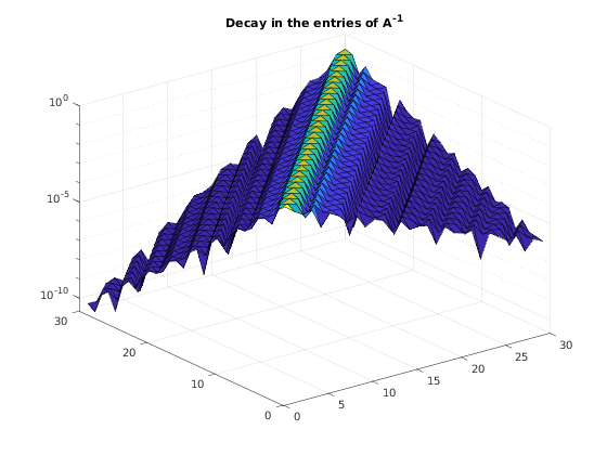
It's importante to notice that in this case the symbol of iA$ is not of finite length, since it is the Laurent expansion of $a(z)^{-1}$. In practice, the toolbox automatically truncate the symbol to the necessary length. We can visualize the exponential decay of the symbol entries by plotting a finite section of the inverse.

surf(abs(iA(1:30, 1:30)));
set(gca,'zscale','log'); % log-scale to appreciate the exponential decay
title(gca, 'Decay in the entries of A^{-1}');

To check how long is the symbol, or how large is the support of the low-rank correction, we may use the command symbol and correction:

[am, ap] = symbol(iA);
nm = length(am), np = length(ap), nc = size(correction(iA))

These lengths are not symmetric because the symbol of $A$ was not symmetric in the first place.

Linear systems

Quite often, we do not need to explicitly compute the inverse, but rather to solve a linear system of the form

$$ Ax = b, $$

where $A$ is QT, and $x$ and $b$ vectors of infinite length. If this is the case, we may resort to computing a $UL$ factorization instead, and solve the system by running the following commands.

b = randn(4, 1);
b = cqt(b); % We interpret b as a vector of infite size.
x = A \ b;
x = correction(x) % Automatically truncate x to the necessary length

Please visit the chapter on linear systems for further details on this matter.

Arithmetic operations between QT matrices

Contents

Additions and multiplications

Computing inverses

Linear systems